Conjoint Analysis on Spotify HK University Student Users
marketing pythonThere are 4 main music streaming service providers in Hong Kong: Joox, KKBox, Spotify and Moov. And here are some basic data of them, just for your information.
| Joox | KKBox | Spotify | Moov | |
|---|---|---|---|---|
| free trial | yes | 7 days | yes | 14 days |
| price/month | 38 HKD | 58 HKD | 58 HKD | 48 HKD |
| student price/month | 31.8 HKD | 29 HKD | 29 HKD | 24 HKD |
| lyrics | yes | yes | no | yes |
| library size | 30 million | 40 million | 30 million | 1 million |
| downloadable | yes | yes | yes | yes |
| highest sound quality | 1411kbps FLAC | 320kbps AAC | 320kbps AAC | 1411kbps FLAC |
| music styles and special features | local HK artists | Japanese, Korean and Chinese songs | European and American songs | exclusive playlists and online concerts |
(source: https://moneyhero.com.hk, July 2020)
survey
In order to discover which attributes influence the customers’ decision the most in terms of selecting a music streaming service, we conducted a survey on the university students in Hong Kong, aging between 18-24, who may or may not uses music streaming service.
The survey was designed to collect data need for a rate-based conjoint analysis. We designed 12 imaginary music streaming service packages, including the attributes mentioned above, and had our participants rate each package from 1-10 based on their own preferences.
dataset
After successfully collected the response from 60 university students, we cleaned and reorganized the dataset using Excel. Next, we loaded the dataset into jupyter notebook using Pandas, and be ready to conduct the conjoint analysis.
tools & skills
- tools: Python, Jupyter Notebook
- skills: Excel, data cleaning with Pandas, visualization with Seaborn and Matplotlib
data exploration & cleaning
First of all, I loaded the needed packages for the analysis, including pandas and numpy.
import pandas as pd
import numpy as np

df = pd.read_csv('data.csv')
df.head()
Because in the original dataset, 'brand' was a categorical variable, we converted it into dummy variables using get_dummies in pandas.
df[['is_joox', 'is_kkbox', 'is_spotify', 'is_moov']] = pd.get_dummies(df.brand)
df = df.drop('brand', axis=1)
df.head()
Likewise, we converted 'sound_quality' into dummy variables as well. Although the feature is numerical, the values of sound quality are not continous. We had to treat them like categorical variables.
df[['sq_256', 'sq_320', 'sq_1411']] = pd.get_dummies(df.sound_quality)
df = df.drop('sound_quality', axis=1)
df.head()
Lastly, we split the DataFrame into y and X features.
y = df['rate']
X = df[['price', 'library_size', 'with_lyrics', 'downloadable', 'is_joox',
	'is_kkbox', 'is_spotify', 'is_moov', 'sq_256', 'sq_320', 'sq_1411']]
conjoint analysis
import statsmodels.api as sm
import seaborn as sns
import matplotlib.pyplot as plt
plt.style.use('bmh')
res = sm.OLS(y, X, family=sm.families.Binomial()).fit()
res.summary()
df_res = pd.DataFrame({
    'param_name': res.params.keys()
    , 'param_w': res.params.values
    , 'pval': res.pvalues
})
# adding field for absolute of parameters
df_res['abs_param_w'] = np.abs(df_res['param_w'])
# marking field is significant under 95% confidence interval
df_res['is_sig_95'] = (df_res['pval'] < 0.05)
# constructing color naming for each param
df_res['c'] = ['blue' if x else 'red' for x in df_res['is_sig_95']]

# make it sorted by abs of parameter value
df_res = df_res.sort_values(by='abs_param_w', ascending=True)
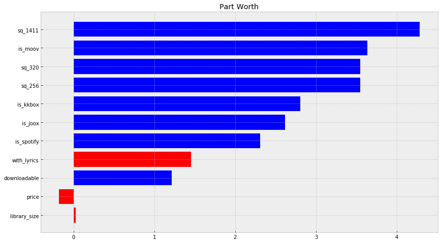
f, ax = plt.subplots(figsize=(14, 8))
plt.title('Part Worth')
pwu = df_res['param_w']
xbar = np.arange(len(pwu))
plt.barh(xbar, pwu, color=df_res['c'])
plt.yticks(xbar, labels=df_res['param_name'])
plt.show()
# need to assemble per attribute for every level of that attribute in dicionary
range_per_feature = dict()
for key, coeff in res.params.items():
    sk =  key.split('_')
    feature = sk[0]
    if len(sk) == 1:
        feature = key
    if feature not in range_per_feature:
        range_per_feature[feature] = list()

    range_per_feature[feature].append(coeff)
# importance per feature is range of coef in a feature
# while range is simply max(x) - min(x)
importance_per_feature = {
    k: max(v) - min(v) for k, v in range_per_feature.items()
}

# compute relative importance per feature
# or normalized feature importance by dividing
# sum of importance for all features
total_feature_importance = sum(importance_per_feature.values())
relative_importance_per_feature = {
    k: 100 * round(v/total_feature_importance, 3) for k, v in importance_per_feature.items()
}
alt_data = pd.DataFrame(
list(importance_per_feature.items()),
columns=['attr', 'importance']
).sort_values(by='importance', ascending=False)
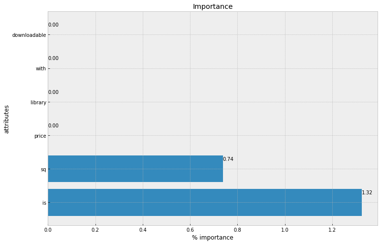
f, ax = plt.subplots(figsize=(12, 8))
xbar = np.arange(len(alt_data['attr']))
plt.title('Importance')
plt.barh(xbar, alt_data['importance'])
for i, v in enumerate(alt_data['importance']):
ax.text(v , i + .25, '{:.2f}'.format(v))
plt.ylabel('attributes')
plt.xlabel('% importance')
plt.yticks(xbar, alt_data['attr'])
plt.show()
alt_data = pd.DataFrame(
    list(relative_importance_per_feature.items()),
    columns=['attr', 'relative_importance (pct)']
).sort_values(by='relative_importance (pct)', ascending=False)


f, ax = plt.subplots(figsize=(12, 8))
xbar = np.arange(len(alt_data['attr']))
plt.title('Relative importance / Normalized importance')
plt.barh(xbar, alt_data['relative_importance (pct)'])
for i, v in enumerate(alt_data['relative_importance (pct)']):
    ax.text(v , i + .25, '{:.2f}%'.format(v))
plt.ylabel('attributes')
plt.xlabel('% relative importance')
plt.yticks(xbar, alt_data['attr'])
plt.show()
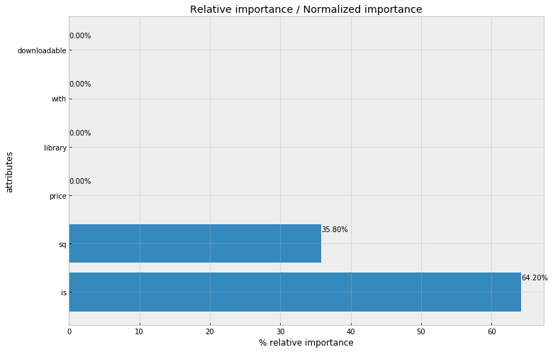
conclusion
'sound_quality' and 'brand' are the 2 most influenctial attributes for university students in Hong Kong when choosing a music steaming service. Suprisingly, 'price' is not one of the important attributes. However, there might be other factors like the music styles and special features that are not measurable in this case. We will be able to investigate into those when more detailed data are collected.
*This report is originally the final team project of the Marketing Analytics (MKTG4090) course at CUHK. I have re-organized and re-analyzed data and created this post. Shout out to my teammates Cathy, Terrence and Alex, thanks guys!